Dense document embeddings often lack contextual information from surrounding documents, which can limit their effectiveness in retrieval tasks. To address this, two complementary methods are proposed: a contrastive learning objective that incorporates document neighbors into the loss function and a new architecture that explicitly encodes neighboring document information. These approaches enhance performance, especially in out-of-domain scenarios, and achieve state-of-the-art results on the MTEB benchmark without complex training techniques like hard negative mining or large batch sizes. The methods can be applied to improve any contrastive learning dataset or biencoder model.
Preliminary.
Text retrieval methods can be viewed probabilistically by computing a distribution over documents using a scalar score function, which matches documents and queries. Vector-based retrieval methods factor the score into two embeddings: one for the document and one for the query. This allows precomputation of document embeddings, facilitating fast retrieval of the top results. Traditional statistical methods rely on frequency-based embeddings, while neural retrieval methods learn dense vectors using training data with document-query pairs. To handle large datasets, contrastive learning is used, where the likelihood of selecting a relevant document is approximated with negative samples and mini-batch examples to optimize the embeddings efficiently.
The approach
Contextual training with adversarial contrastive learning
In document retrieval, terms that are rare in general training datasets may be common in specific domains, making standard training less effective. To address this, a meta-learning-inspired objective is used, where documents are grouped into fine-grained pseudo-domains for training. These groups are formed using clustering to find challenging configurations based on document-query similarity. The clustering problem is framed as an asymmetric K-Means task, minimizing distances between pairs and centroids.
False negatives, which can disrupt training, are filtered out using equivalence classes defined by a surrogate scoring function. The final step packs clusters from within the same domain into equal-sized batches, introducing randomness in training. This approach enhances the model’s generalization by simulating domain-specific variations during training.
Contextual document embeddings
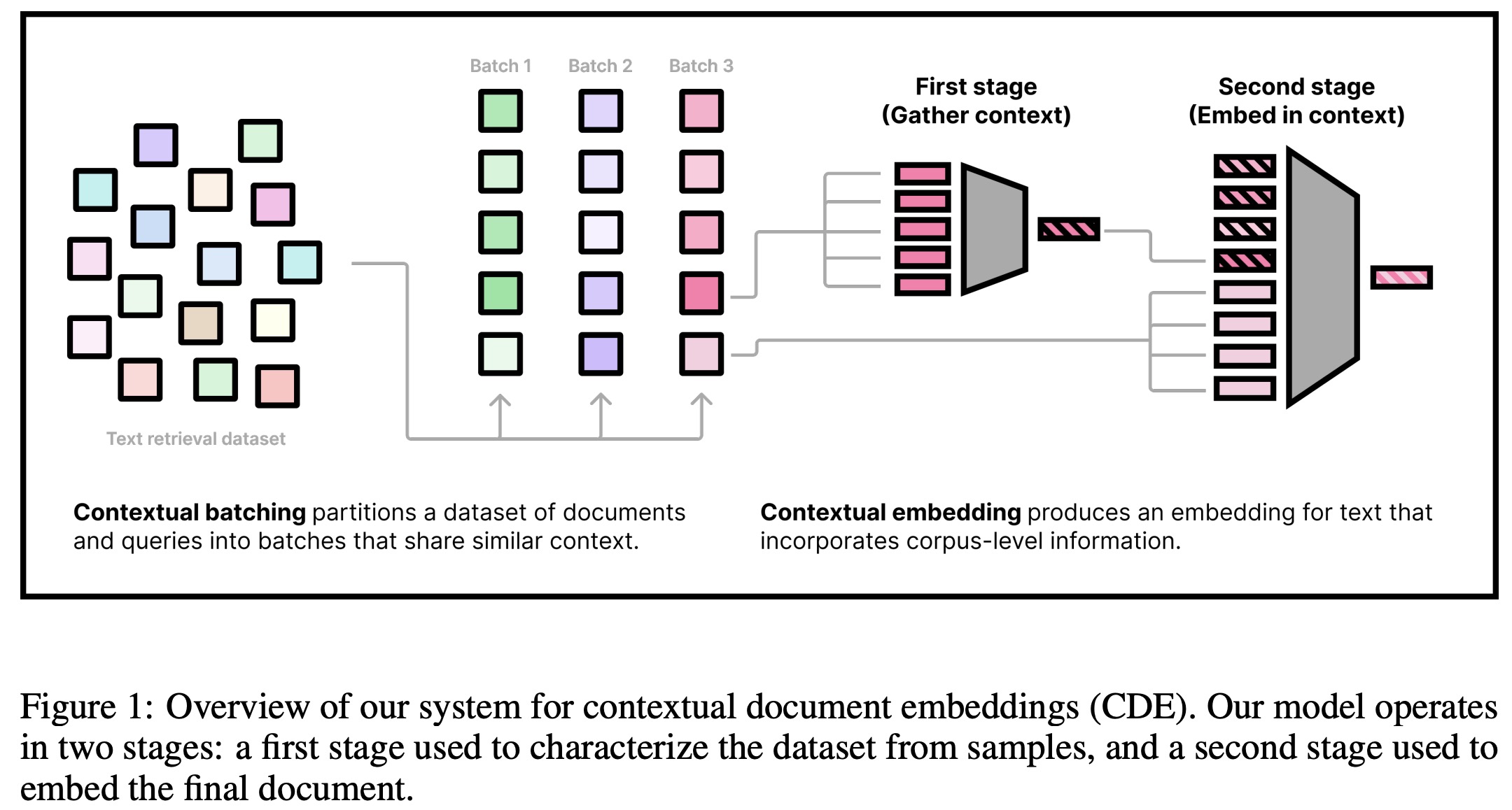
The authors introduce a two-stage architecture to add contextualization directly into document embeddings, inspired by traditional approaches that utilize corpus statistics. The goal is to allow the model to learn contextual information without having full access to the entire dataset, balancing efficiency and effectiveness.
- First Stage: Pre-embed a subset of the corpus using a separate embedding model to gather contextual information. These context embeddings are shared within a batch, reducing computational costs.
- Second Stage: Compute the document embeddings by combining the context embeddings with the document tokens, using a second model.
A similar approach is used for the query encoder, but only documents provide context since queries typically lack context at test time.
To improve generalization, the model uses sequence dropout, replacing some context embeddings with a null token to handle scenarios with limited or unavailable context. Positionality is removed to treat the documents as unordered.
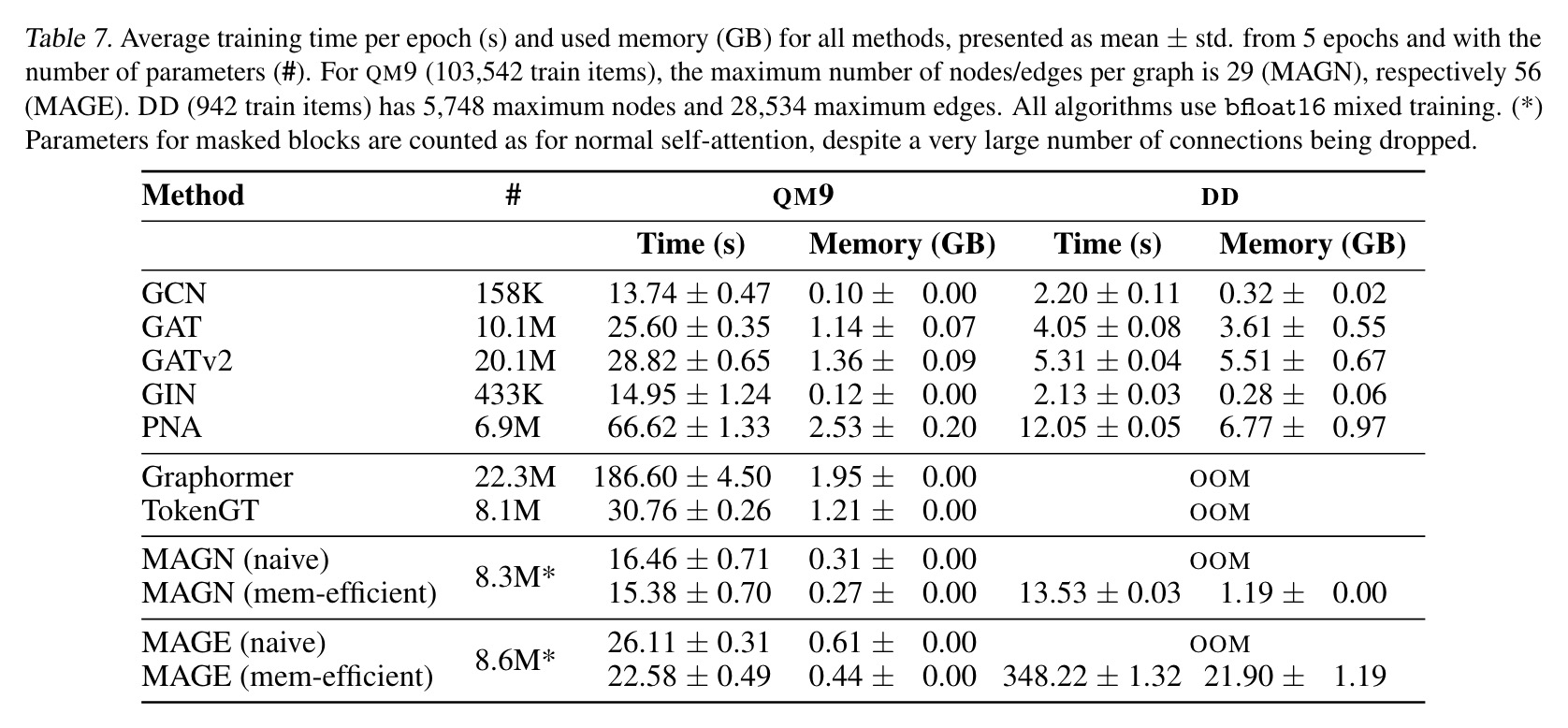
For efficient training, the model employs a two-stage gradient caching technique, enabling larger batches and more contextual samples without memory issues. This approach calculates gradients separately for each stage, freezing representations initially and then backpropagating through the second stage, allowing a tradeoff between computation and memory.
Experiments
The authors perform experiments with both small and large configurations. In the small setup, a six-layer transformer with a maximum sequence length of 64 and up to 64 contextual tokens is used to evaluate on a truncated version of the BEIR benchmark. They explore different batch sizes ranging from 256 to 4096 and cluster sizes up to 4.19 million. Training follows the typical two-phase approach: a large unsupervised pre-training phase followed by a short supervised phase.
The implementation uses the GTR model with clustering algorithms based on FAISS, and training initializes the two-stage models with weights from BERT-base.
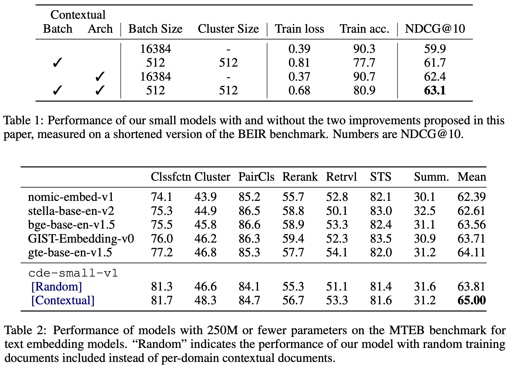
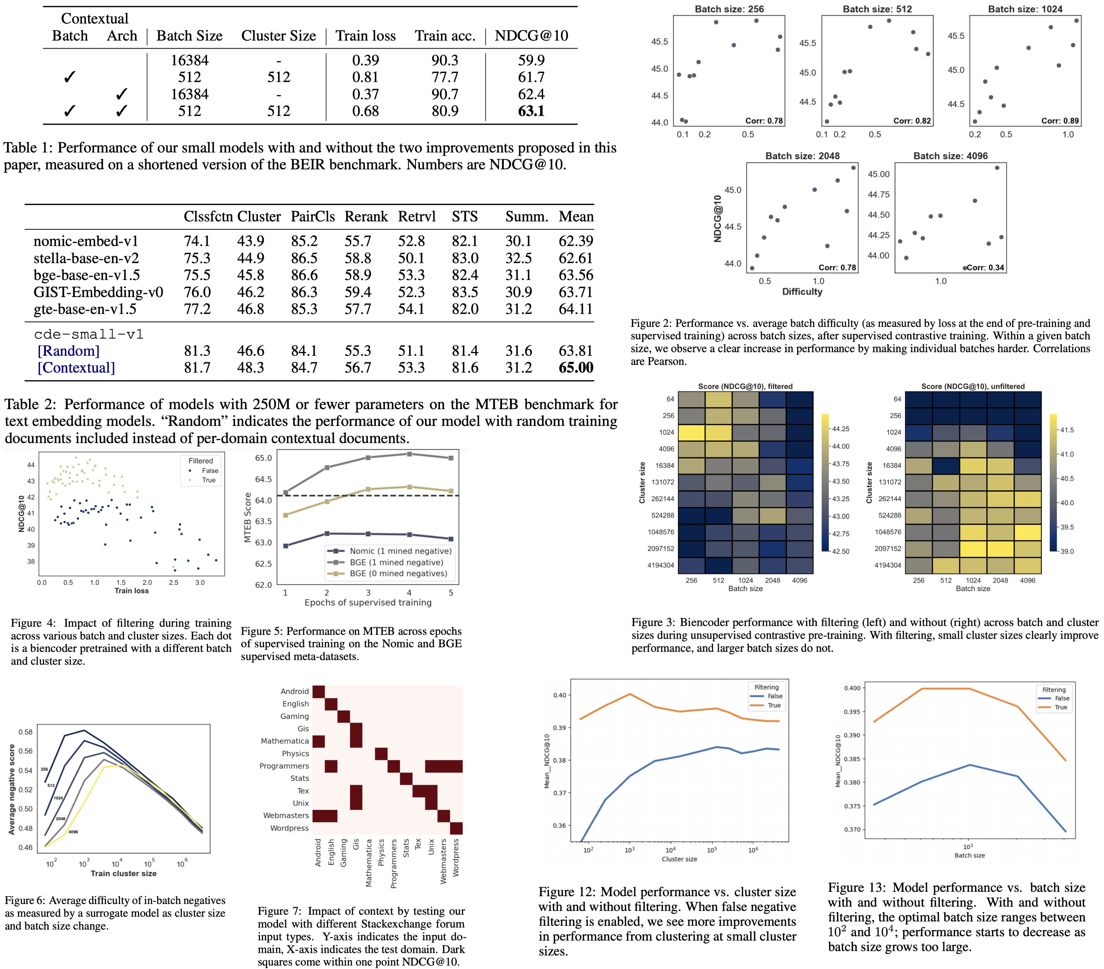
The results prove the effectiveness of combining adversarial contrastive learning with a contextual architecture for improving document retrieval models. In smaller experiments, both techniques independently showed improvements over standard biencoder training, with the largest gains seen when combined.
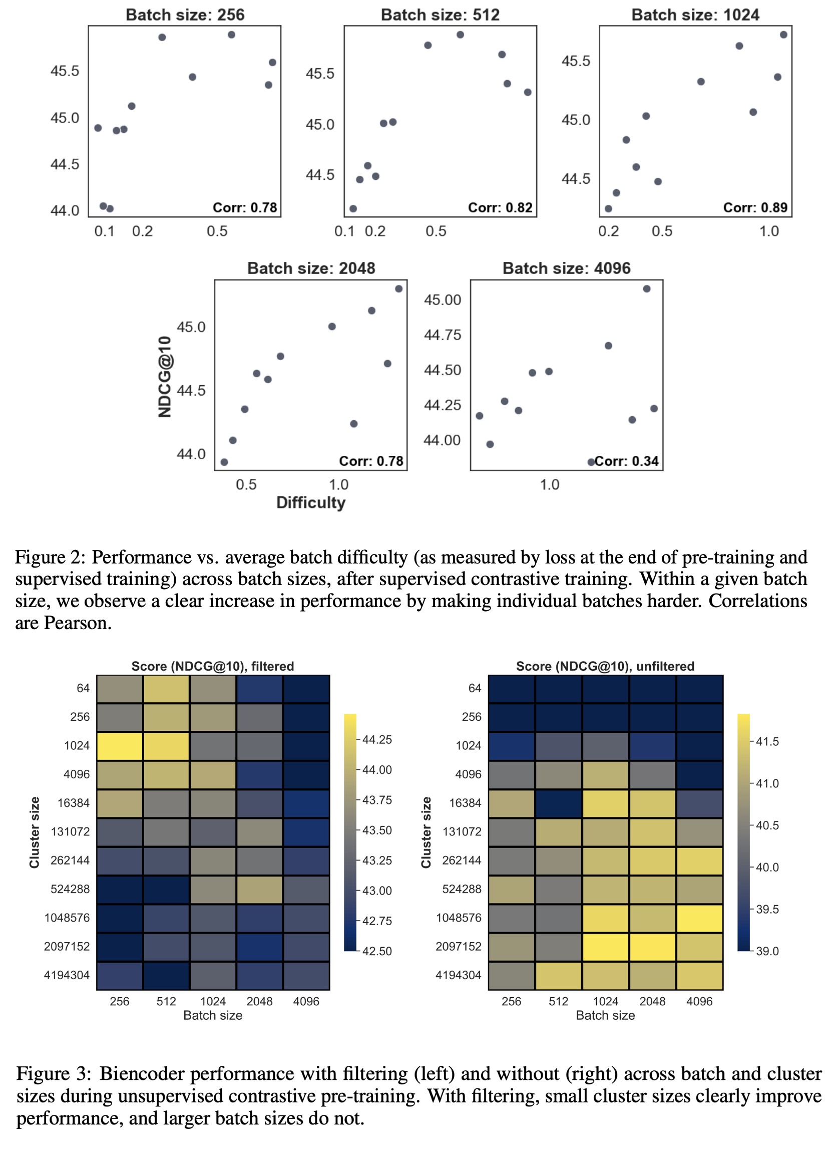
The use of contextual batching revealed a strong correlation between batch difficulty and downstream performance. Reordering datapoints to create more challenging batches enhanced overall learning, aligning with previous research findings. Additionally, filtering out false negatives improved model performance significantly.
The experiments compared the contextual architecture to a biencoder across multiple datasets from BEIR. The contextual approach consistently matched or outperformed the biencoder, especially in smaller or out-of-domain datasets like ArguAna and SciFact.
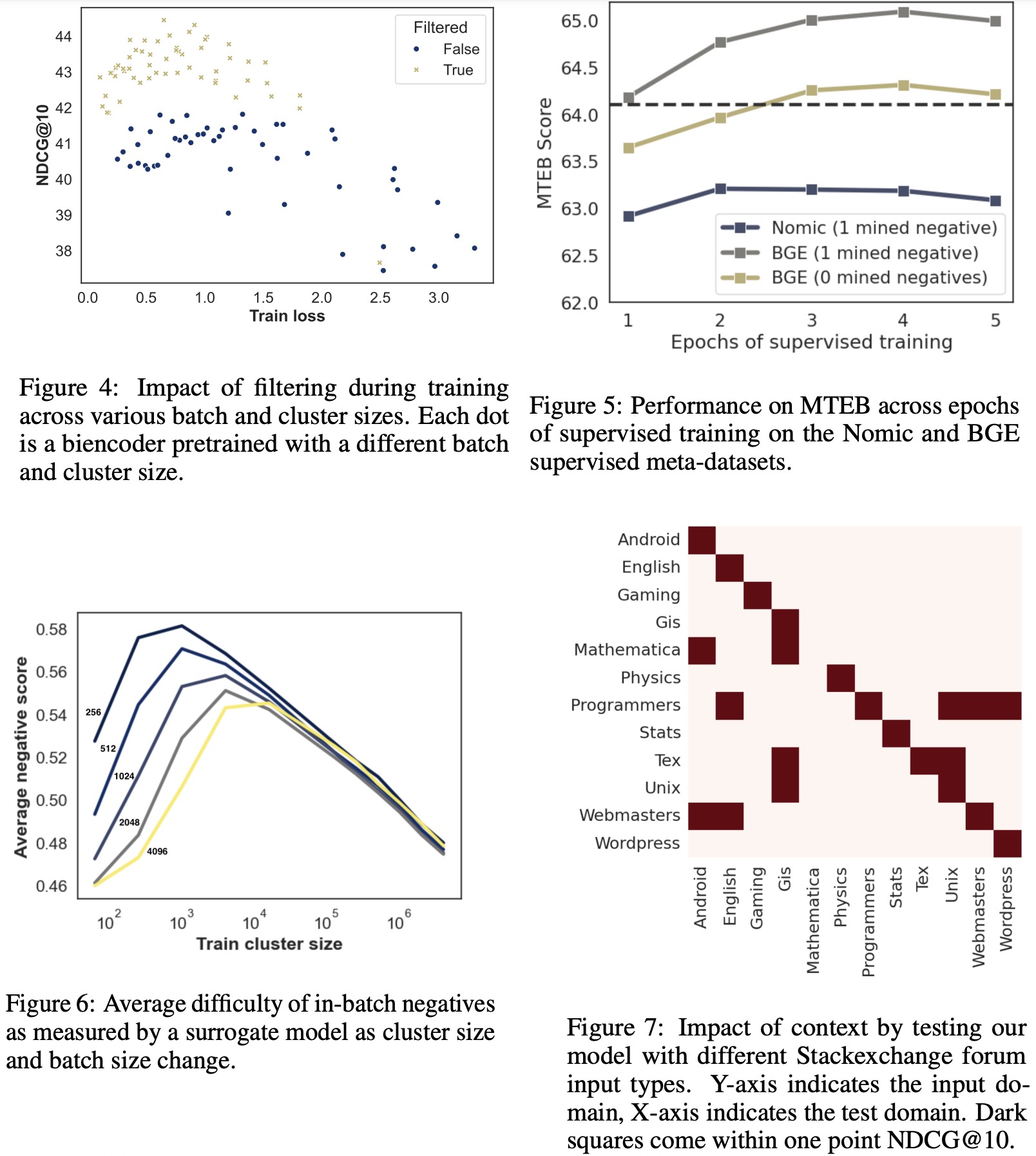
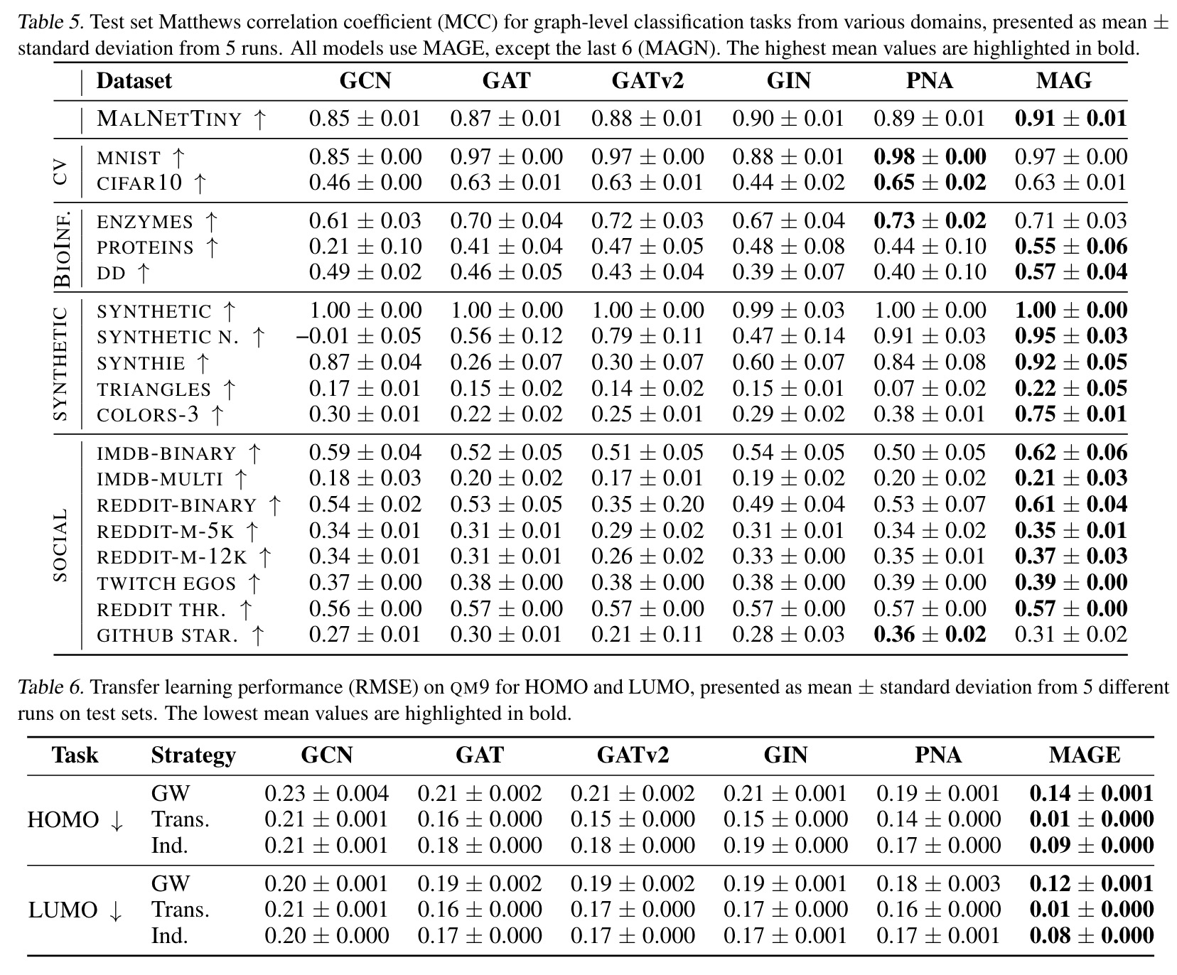
Full-scale training with multiple epochs demonstrated optimal performance after four epochs on the BGE datasets. The best supervised model, cde-small-v1, achieved state-of-the-art results on MTEB without relying on multiple hard negatives per query. The model also showed improvements in non-retrieval tasks like clustering, classification, and semantic similarity.
In scenarios with limited context (simulated using random documents), there was an average performance drop of 1.2 points, indicating the model’s dependency on contextual information for optimal results.
]]>