Cayley graph search with Claude Code: what puzzle competitions look like in 2026
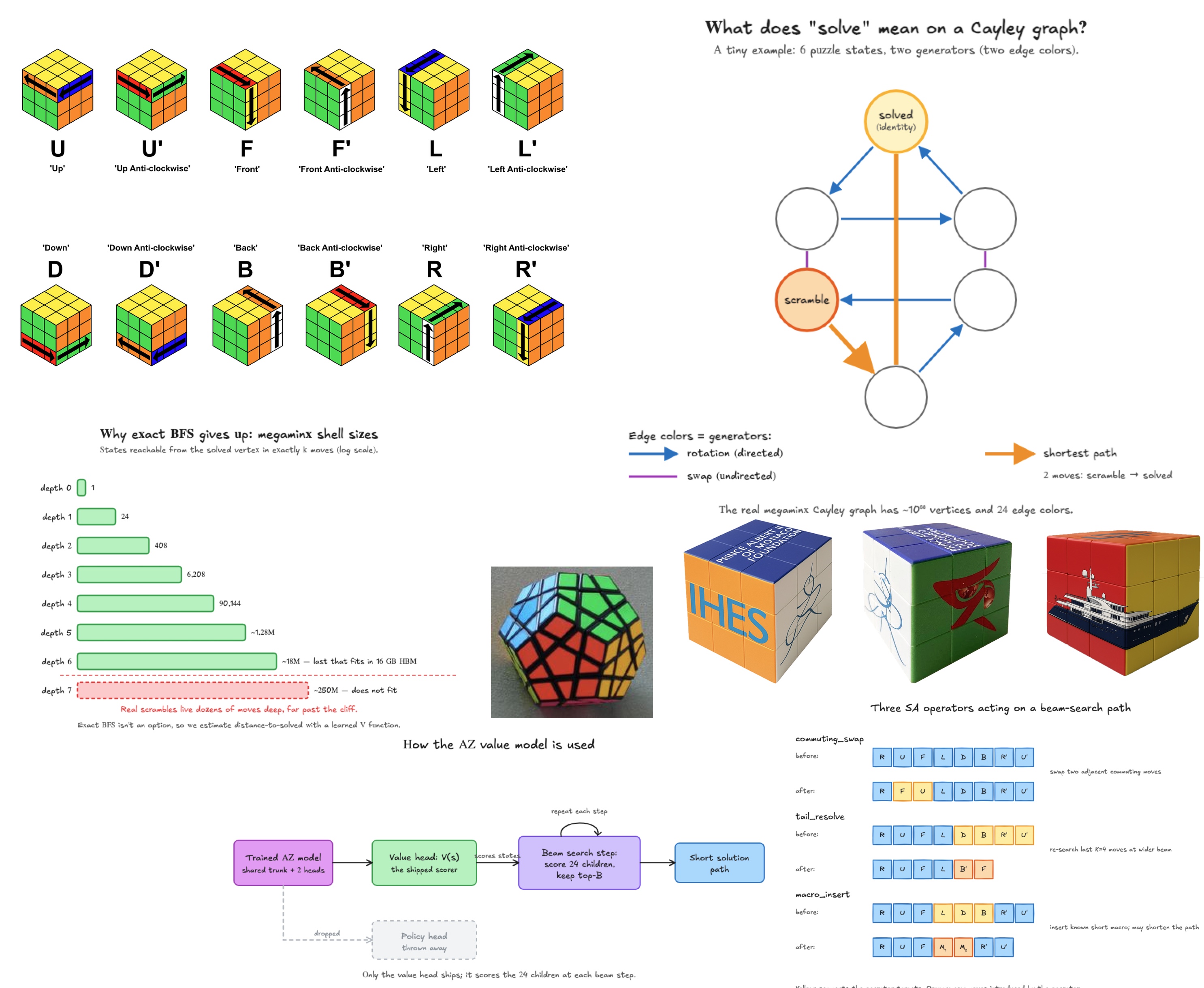
Over the last couple of months, I worked on two Kaggle competitions in the CayleyPy series: IHES Picture Cube and Megaminx. Both are combinatorial puzzle solvers, and they can be reformulated as a search in an enormous implicit Cayley graph: each puzzle state is a vertex, each possible move is an edge, and solving means finding a short path back to the identity. This is a long term-activity: we have been researching these puzzles for a couple of years and have published several papers. This year we took another step toward solving them.
I remember working on this in 2024. At that time, all code was written by hand, and I spent a lot of time debugging it and digging into documentation. But much has changed in these two years: nowadays, agentic workflows are a significant part of my workflow, and I can delegate much of the implementation work to an LLM, focusing on decisions rather than specifics (even though I still have to review them).
I used Opus inside Claude Code as the implementation agent for both competitions. Claude wrote essentially all of the training scripts, beam-search variants, TPU ports, submission automation, and post-processing tools. I still reviewed the code, checked outputs, and made the experiment-level decisions. I focused on guiding it and preventing it from going too far down the wrong path (which it did quite often): I told it which ideas to try, which areas to research, when to stop iterating on a dead-end model, when to pivot, etc.
So this post is about two things. One is about working with Cayley graphs: how to combine learned distance heuristics, wide beam search, symmetry, and path post-processing to solve puzzle graphs far too large to search with DFS/BFS. The second one is about agentic workflow: what it actually looks like to run a research loop when an agent handles implementation and the human role shifts toward experimental design, plateau detection, and search strategy.
I share the scores reached by different methods as a proxy of progress. The leaderboard shows a single number (total moves over a fixed set of scrambles), but it is the logic behind the solutions that matters. Score improvement indicates we were able to find shorter paths, so higher places on the leaderboard reflect a better understanding of the search problem.
What’s a Cayley graph, and why would you solve one?
Let’s start with an explanation of what a Cayley graph is and how we can work with it.
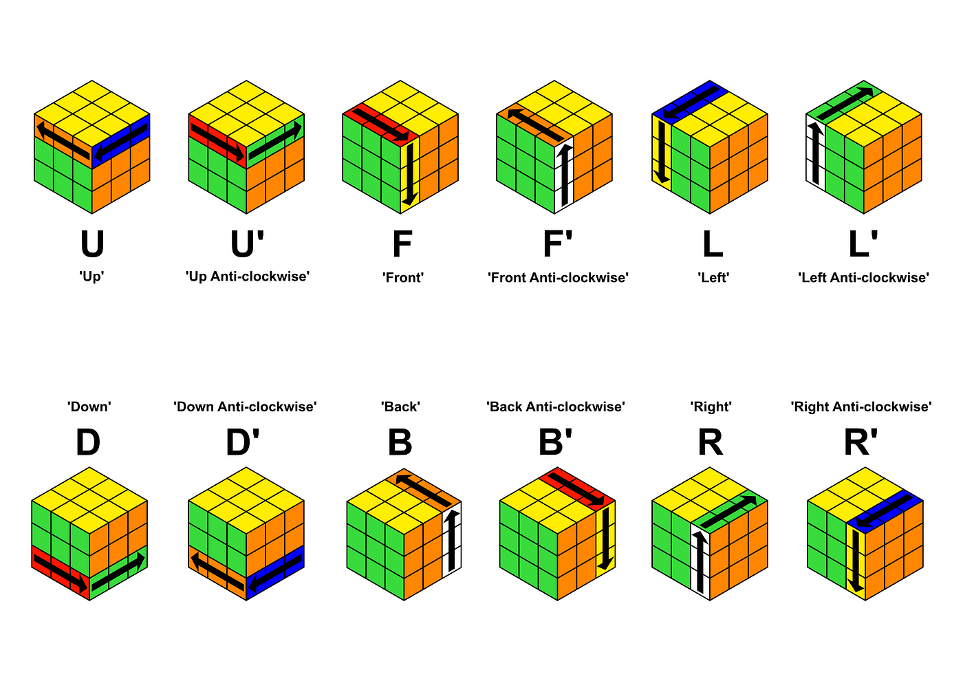
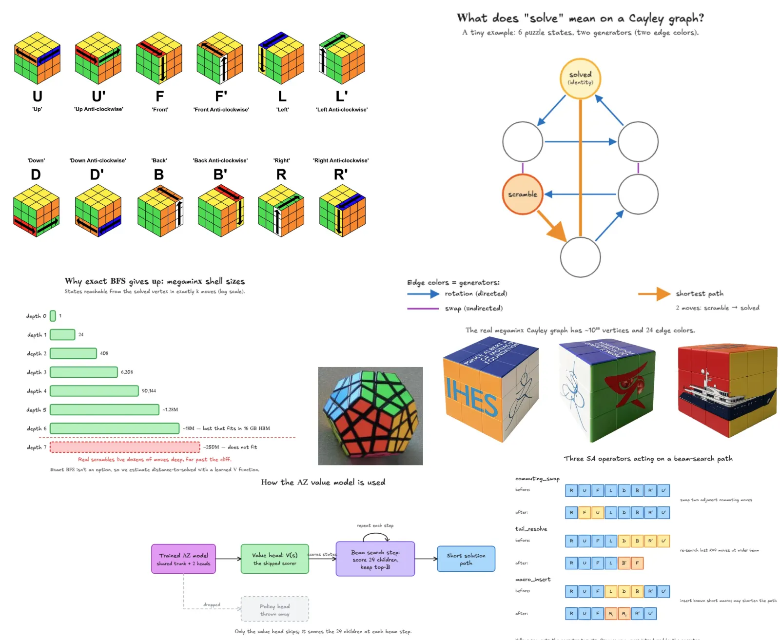
We have a puzzle (like a Rubik’s cube). Possible moves (generators) are a small set of operations (like turning a face of the cube). The puzzle has a solved state, and we can scramble it by applying a sequence of moves. The goal is to find a sequence of moves that returns the puzzle to the solved state.
In a Cayley graph, we have one vertex per element (every reachable configuration of the puzzle), and an edge between two vertices whenever a single generator takes one to the other.. The solved state is the identity vertex; a scramble is some other vertex. Solving the puzzle is finding a path from the scramble back to the identity, and solving it well (the score that we care about) is finding a short one. The shortest possible path is the scramble’s true distance-to-solved; the largest such distance over all scrambles is the graph’s diameter, known to cubers as “God’s number”.
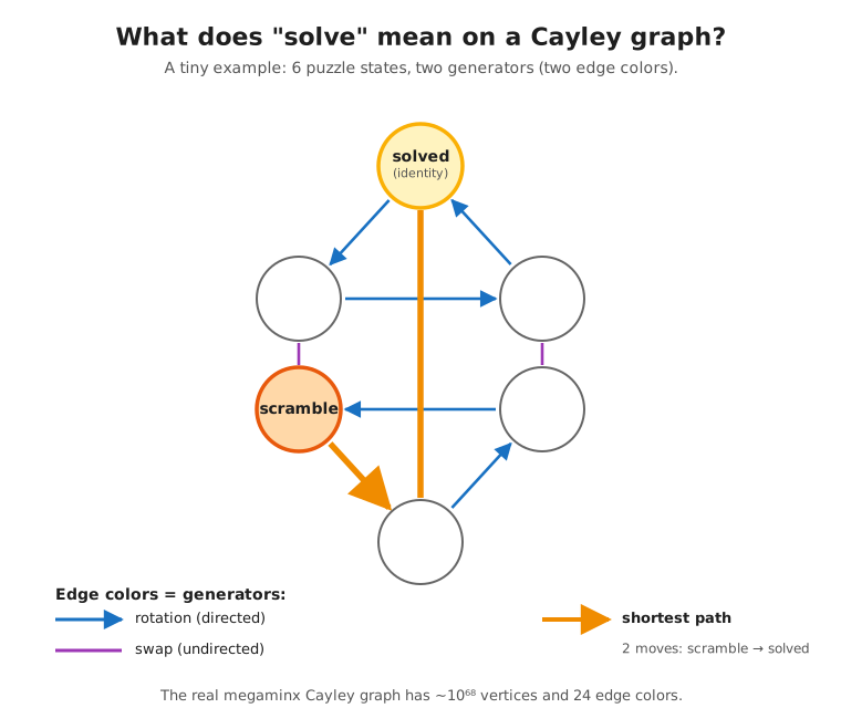
By Cayley’s theorem, every finite group is a group of permutations, so permutation puzzles are a concrete handle on finite group theory in general.
The significance of Cayley graphs
A Cayley graph is one of the standard ways of representing a group as a geometric object: vertices are elements, edges are generators, and the graph metric becomes a distance measure in the group. This is why these competitions combine discrete optimization with geometric group theory. The basic questions are genuinely hard — nobody proved the 3×3×3 cube’s God’s number is 20 until 2010, and the value for megaminx is unknown.
Why a brute search can’t solve it
These graphs are far too big to write down. The 3×3×3 cube has about 4.3 × 10^19 states; the megaminx has roughly 10^68, astronomically more. In practice, you don’t even try to store the graph — you keep one state and generate its neighbors on the fly. The graph is defined implicitly, by its generators.
Breadth-first from solved is fine for a few moves — on megaminx. the numbers of states are 1, 24, 408, 6208, 90144, 1.28M, then ~18M states at depth six — but depth seven is ~250M, and a real scramble is dozens of moves deep.
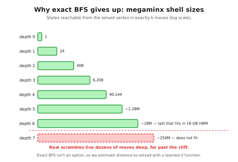
So you can’t compute the true distance-to-solved; you estimate it with a learned heuristic and search against it. The whole problem boils down to two questions: how good is the estimate and how wide a beam can you afford. And one unfortunate consequence is that achieving the best results often means cramming the largest possible beam onto a TPU.
CayleyPy, IHES, and megaminx
CayleyPy is the umbrella for this line of work on finding short paths in Cayley graphs, using learned heuristics and beam search instead of the hand-built solvers that cubers traditionally use. It spun off a series of Kaggle competitions, each a different graph, implemented in the open-source CayleyPy library.
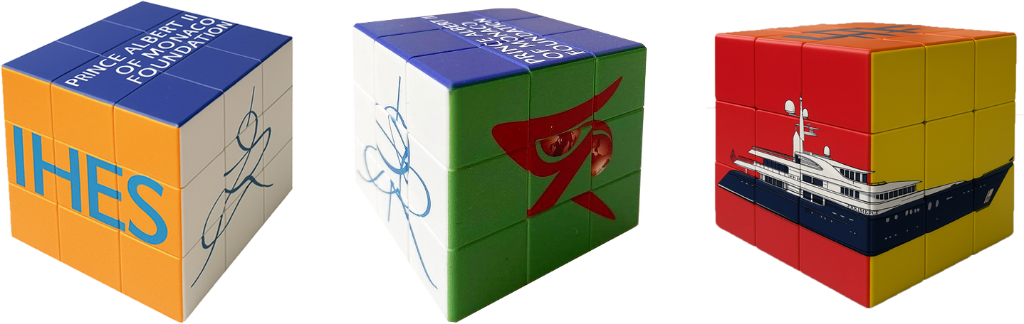
The main puzzle is the IHES Picture Cube: a 3×3×3 with every face distinct. This puzzle is more complex than Rubik’s Cube, as the orientation of the pieces matters, even the centers. There are 1003 scrambles to solve as short as possible. It is named after the Institut des Hautes Études Scientifiques outside Paris, the institute where Mikhail Gromov, the one who turned the study of groups into the geometry of their Cayley graphs, has spent his career.
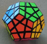
Megaminx is not a cube but a dodecahedron with twelve pentagonal faces turning in fifths of a full rotation. My solver encodes a state as a length-120 vector with 24 generators (12 faces × 2 directions), and the competition provides 1001 scrambles.
Megaminx is an interesting challenge for two reasons. First, there is no strict algorithm to fall back on (unlike the smaller puzzles where I could use a Kociemba-style two-phase solver), so learned-heuristic search is basically the only viable approach. Second, because the total score is calculated over a thousand scrambles, even small improvements can provide a visible improvement.
I had modest computational resources: a 16 GB RTX 4090 laptop as my primary device, a GCP L4 machine for long jobs, free Kaggle GPU and TPU kernels for parallel exploration, and later I got access to a larger TPU kernel. I got free GCP credits thanks to being a Google Developer Expert, and they helped us run heavy jobs on GPUs and wide-beam search on TPUs.
The core approach
Both competitions follow the same approach, and the focus is on making it work better, faster, and more efficiently:
- Train V(s), a neural estimate of distance-to-solved, on random walks from the solved state.
- Run beam search, using V to rank children and keep the best B at each step.
- Solve each puzzle in decorrelated ways: different beam directions, symmetries, and search configurations.
- Post-process the completed paths to shorten them.
- Min-merge every solution, keeping the shortest path per puzzle. Merging solutions created by different people is often a key to significantly improving the score.
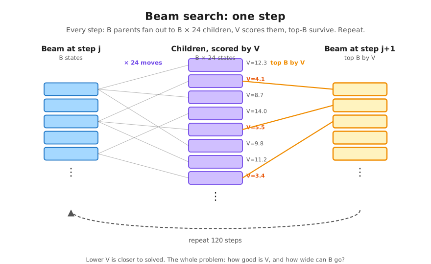
This approach is straightforward, but each stage can be complex and computationally expensive to run. Here is what the Claude role was in each stage of the search loop:
| Component | Role in search | What Claude contributed |
|---|---|---|
| V(s) model | ranks states by estimated distance | quick architecture and training variants |
| Beam search | turns the heuristic into paths | fast ports and memory optimizations |
| Directional / symmetry variants | decorrelate failures | easy to implement and batch |
| Path post-process | improves completed solutions | quick SA (simulated annealing) and post-processing prototypes |
| Min-merge | keeps only the shorter valid paths | automated verification and submission |
The rest of the post is about my approaches to improving the solutions for both competitions.
The scaffolding
Over the course of the two competitions, I built a scaffolding that let me run the research loop with minimal intervention. I needed a solution that could survive context resets when starting new sessions, track long-running jobs, and keep work state in a single place.
There were three main parts:
- Markdown state files.
IDEAS_CATALOG.md,EXPERIMENTS.md,HANDOFF.md. Claude Code session lose context when the sessions is too long or when you end it, so anything important was written down into one of these files. - Slash commands for repeated tasks. At first, I created commands to quickly upload submissions to Kaggle; then added commands to check job status, merge submissions, and more.
- Background tasks and Monitor for long jobs. I often had to launch many hour-long runs (sometimes more than 24h), and needed to monitor them to make sure they don’t fail or get stuck - Claude was able to manage it.
One of my favorite parts was giving a command like “run this training script on GCP GPU and report the results”; Claude then could spin up a VM, run the job, and show the results. It saved me a lot of time.
I have published the clean code and agent settings here - my working repo is private as it is a mess.
IHES — creating and polishing the core solution
In the IHES Picture Cube, a state is a permutation of 72 stickers (8 corners × 3 + 12 edges × 2 + 6 centers × 4), with 18 generators structured as 3 axis families × 3 layer indices × 2 signs. An adapted Kociemba two-phase solver (a classical computer algorithm for solving a 3x3x3 cube) gave 42718 moves. For a comparison: on the 3×3×3, God’s number is 20, so an “optimal on every puzzle” solver would score ~20k.
| Submission | Score | Main change |
|---|---|---|
| baseline | 42718 | Kociemba two-phase solver |
| 2 | 30770 | real residual blocks in the V-network |
| 3–8 | 27106 | embedding encoder, fast training recipe, wider beam, BFS-d5 |
| 9 | 24998 | 1.6M-param V + Khoruzhii beam searcher |
| 11 | 24068 | Bellman refinement + NISS |
| 12–15 | 23858 | wider-beam tail re-solves |
| 16 | 23672 | int8 state encoding |
| 17 | 23322 | Q-distillation, beam-1M |
| 18 | 23224 | beam-4M full solve + tail re-solve |
From baseline to a small architecture
The Claude library provides a small MLP distance heuristic and a beam search. Claude analyzed the baseline architecture (a sequential MLP) and rewrote it, adding residual blocks, an embedding encoder, a faster training recipe (bf16, torch.compile, fused AdamW, larger batches, 3× throughput), a wider beam, and BFS-d5 post-processing. This improved the score to 27106.
And at this point, I had already noticed the limitations of using agents: the MSE loss wasn’t improving, and after several attempts, the agent started training variations of the same model and ensembling them (just like a real Kaggler aiming for fast score improvement!).
I had to explicitly tell Claude to stop iterating on the same architecture and go after a better single model. I asked it to do deep research on specific topics, and we found multiple relevant works. The next best idea turned out to be not a model improvement but a beam-search improvement. At that point, I was running a beam search with a beam width of 8K, and the GPU memory was already fully used. Claude implemented multiple optimizations (priority-queue-free top-K via torch.topk, contiguous beam buffers reused across steps, and others), which allowed to increase the beam width to 65K, which improved the score by 2k point. This proved that beam search width often plays a more important role than the model architecture.
Bellman, NISS, and the search improvements
As mentioned before, models are usually trained on random walks starting from the solved state, and the labels are the walk depth. But these labels are merely an upper bound on true distance, because the random walk that produced a label might not be optimal. Bellman self-bootstrap (target(s) = 1 + min_a target_net(apply(s, a))) reduces that bias. Adding it helped solve several very hard puzzles.
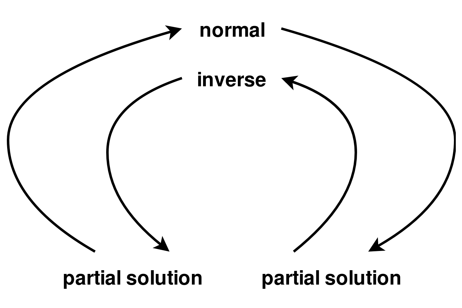
NISS was another noticeable improvement. I asked Claude to mine the speedcubing forums, and it encountered NISS - Normal-Inverse Scramble Switch. Given a scramble, you solve the inverse problem, then reverse the resulting path and invert each move. The expected length is the same, but we have different hash seeds and tie-breaking, so the search is directionally decorrelated. It was simple to implement, and together with Bellman, the score reached 24068.
This is an old idea in the cubing community, but I didn’t even know I could search for it.
The next improvements were incremental: running wider beam search for the hardest puzzles, optimizing beam search (int8 state encoding) to run at 2M width, and Q-function distillation (from Vlad Kuznetsov’s writeup) improved the score to 23322.
Q-function distillation is a very interesting trick: you train a network with 18 outputs, the i-th predicting V(apply(s, action_i)); one forward pass then gives all 18 neighbor scores (no need to run 18 passes), and children are generated only for the top-B among the 18·B candidates. That was an ~8× speedup at beam 524K, and it cuts beam memory as well as time.
The final solution was a combination of all the above and took ~9 hours to run training and 4M beam search on a GCP L4. I min-merged it with my previous best submission and got 23224 moves, about 1400 moves behind Tomas Rokicki.
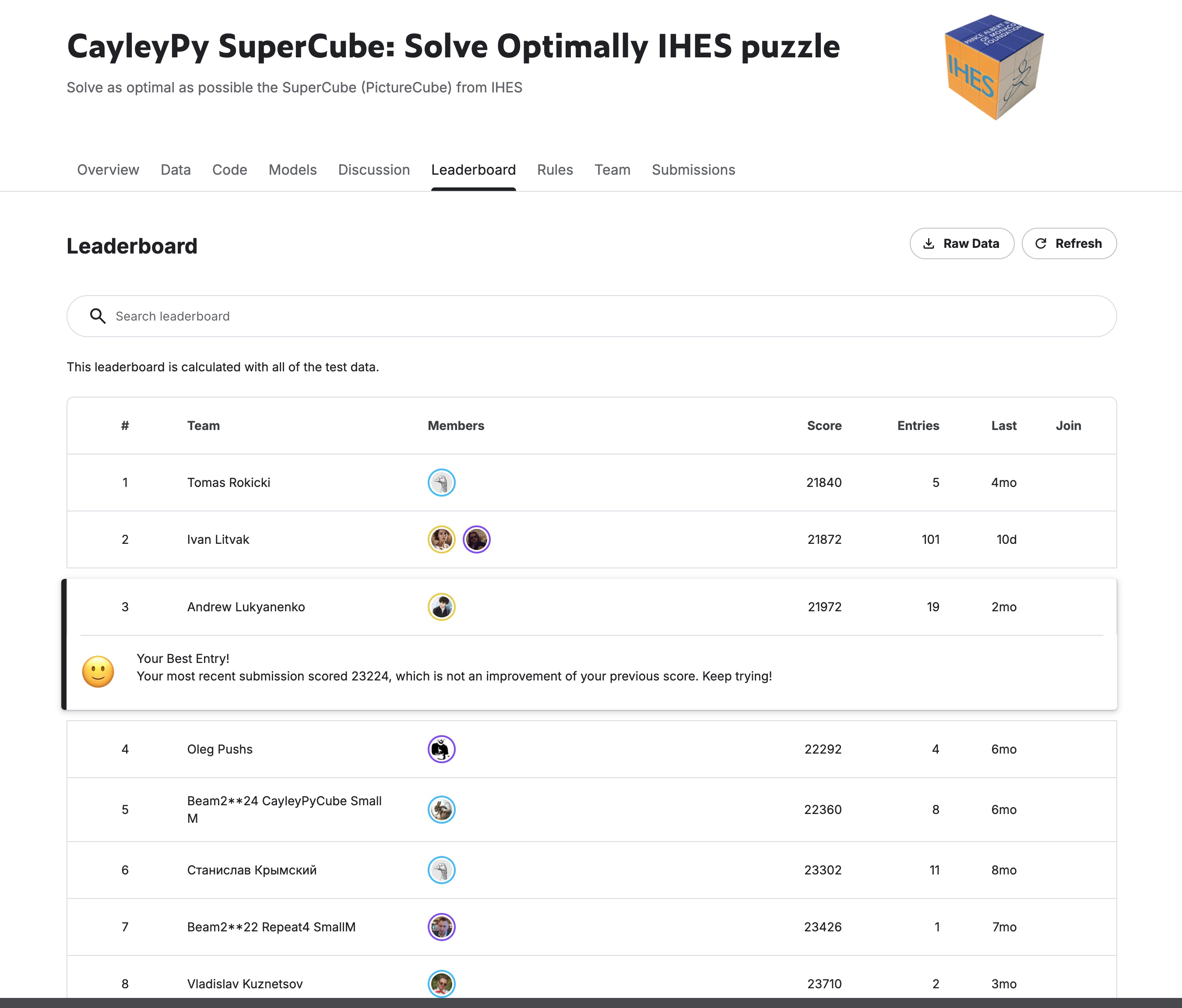
Min-merging my solution with the best public one gave me 21972, but I don’t count it as my own - this is a team effort.
What didn’t work
I have tried a lot of ideas, and many didn’t work; for example, training larger models produced worse results.
- A piece-decomposition input encoding trained worse than the flat 72-sticker embedding and ran 2.5× slower at inference.
- 24× rotational symmetry augmentation converged like the baseline and didn’t beat the previous record.
- A commutator-library window-replacement pass had zero hits, because beam paths aren’t commutator-structured the way hand-written FMC solutions are.
- BFS-d6 window replacement gave nothing over d5.
- A twips/twsearch integration would have been days of work for uncertain payoff.
The result: model improvements over the small-arch + Bellman + n_back=1 didn’t help. Most of the improvements came from improving the beam search.
Megaminx — reusing and improving the previous approach
| Submission | Score | Main change |
|---|---|---|
| baseline | 415521 | post-processing only (no model) |
| 2 | 407563 | first ML V-model (6M embedding ResMLP) + NISS |
| 3–4 | 95682 | full GCP two-pass solve (Bellman-refinement on misses) |
| 5 | 88195 | full beam search 131k + beam-stack rescue |
| 6–10 | 82481 | hard-tail Q-shortlister + beam-524k + sym-ensemble K=2→8 + TensorRT |
| 11 | 82225 | TPU beam, full-1001 (xmp.spawn, K=4) |
| 12–18 | 79522 | tail re-solve + SA local search + wider TPU beams (B up to 1M) |
In Megaminx, we have 12 faces, ~120 stickers, 24 generators (12 face rotations × two directions), and the same metric (total move count) across 1001 test puzzles. I reused most of the code and soon reached 82481. As a comparison, Tomas Rokicki’s score was 93606. This shows that while in smaller puzzles heuristics can be better than search, in larger puzzles search works better.
The first plateau
After the first success, I soon realized that I had reached the plateau. Claude tried 13 variations of Bellman training, but all of them had similar loss. The agent was happy to continue iterations, so I had to stop it and started researching.
Sym-ensemble: 360 rotations as a single model
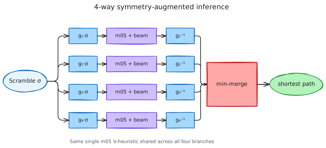
The first breakthrough idea was symmetry-aware ensembling. The megaminx has 360 rotational symmetries (the A₅ × C₆ group acting on the dodecahedron). For a given scramble σ, every rotation g maps it to a rotated scramble g·σ that has the same optimal length; solving each rotated version and inverting back gives many valid paths per puzzle, of which we keep the shortest.
Using all 360 would be too computationally expensive. But even using just four of them was enough to push the average path length from ~89 to 88.20 — a nice improvement without retraining the model.
TPU for a wider beam
As it was mentioned before, increasing the beam width was the most productive lever in IHES. The same was true for megaminx, but I wasn’t able to go past 2-4M on GPU. TPU kernels have much more memory, so I decided to use them and asked Claude to port beam search to TPU.
It took several attempts to get right, but eventually we had a working TPU beam search on Kaggle’s free v5e-8. But it had only 1m width, which was even smaller than the 2-4M I had on GPU.
To make it better, I had Claude shard the beam across all 8 cores of one TPU — shared-beam SPMD, hash-partitioned so that per-step memory is bounded by the local shard rather than the global beam, which lets one beam grow far larger than any single core could hold. And here I hit a hard wall with Claude - it couldn’t implement it correctly after 5 attempts using PyTorch-XLA and 5 attempts using JAX. I asked Codex to review the attempts and suggest fixes, and it produced a working version on its first attempt! This shows that sometimes an agent just doesn’t have sufficient capacity to implement a complex idea, and another agent can do it better.
The problem was in a cross-rank reduce running inside the per-step JIT’d body; moving it onto the host resolved the issue. After that, Codex worked on a few rounds of memory optimization and pushed the shared beam from 8M to 48M states on Kaggle’s free TPU v5e-8, and later to 256M on a bigger v6e-8 TPU on GCP. I will share more details in a separate blogpost.
AlphaZero without self-play: breaking the model ceiling
The previous improvements (sym-ensemble, wider TPU beam with shared-beam SPMD) improved the search, but I was stuck on the model side. I have tried many variations of the model, but the final results (the lengths of the found paths) were roughly the same - ~89 on average on a small 51-puzzle validation set. This led me to conduct in-depth research into alternative directions. Multiple approaches didn’t work (GFlowNets, dataset distillation, admissibility-aware losses), but one did help me improve the score - AlphaZero.
I have used only the architecture part (no MCTS or self-play): a shared trunk with two heads (a 24-way policy head and a scalar value head) trained on a joint CE(policy) + MSE(value) loss. The policy learned by imitating strong solution paths; the value followed the Bellman recipe.
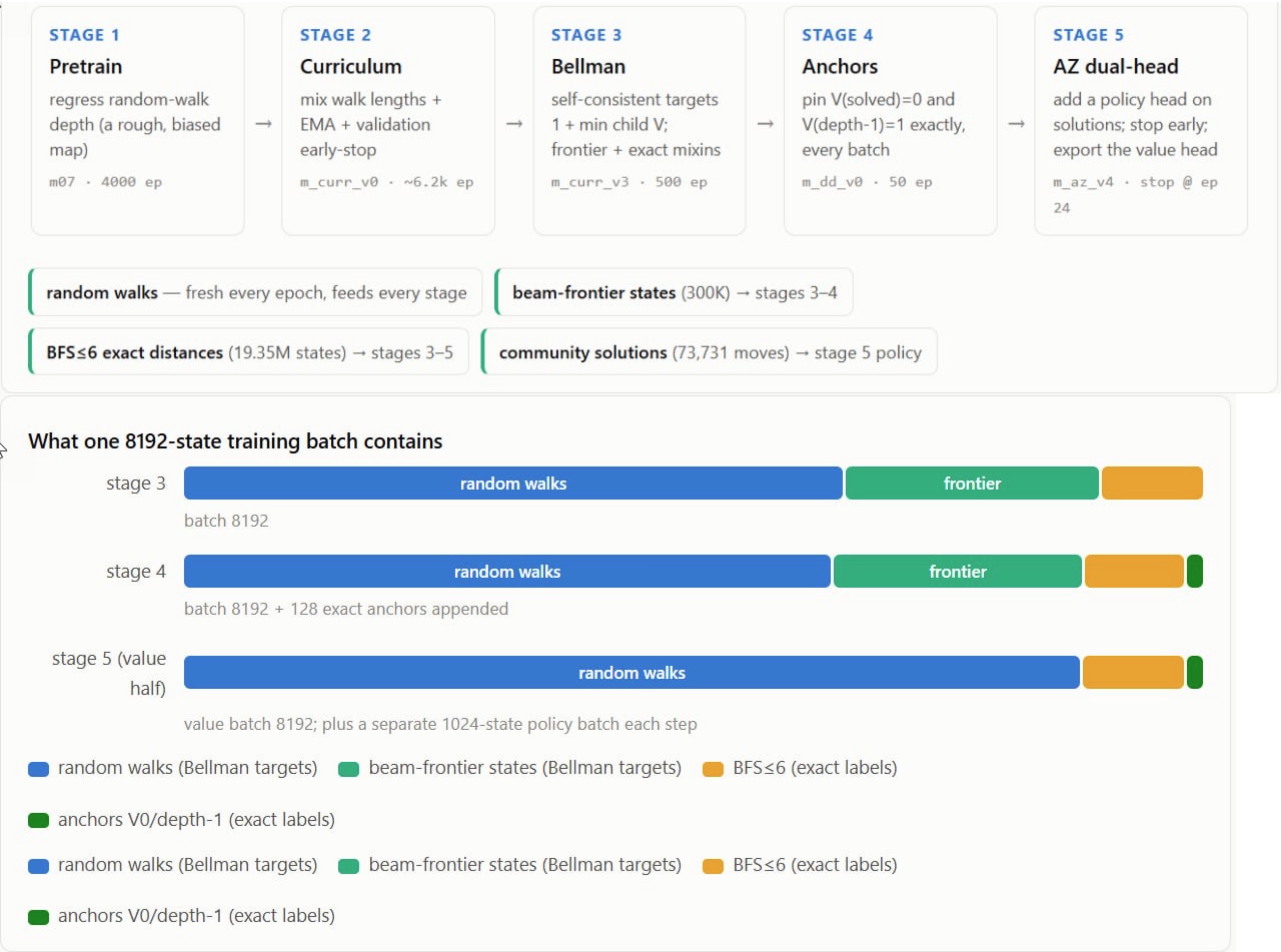
It took several attempts to make it work: I had to retrain the whole pipeline from scratch and mix different types of labels. One more important thing: training longer usually hurt the value head, so I had to stop early. The epoch-24 checkpoint decreased the mean path length down to 87.5.
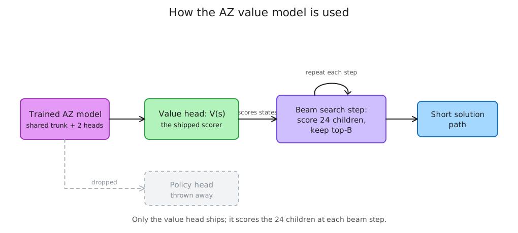
The interesting thing was that while the policy head was useful for training, it was not useful at inference. It helped produce a better value function, but for inference, I used the value head itself directly. The full five-stage training pipeline is reproducible in a public Kaggle notebook.
Simulated annealing on completed paths
Another new thing useful for megaminx was post-processing. I took the completed beam path and tried to hill-climb on it. Claude built a simulated-annealing pass with three operators:
commuting_swap: swap adjacent moves that commute (act on disjoint stickers), which occasionally finds a shorter local segment.tail_resolve: re-run beam search on the last K moves with a wider beam.macro_insert: try inserting known short macros (commutators, fixed-period sequences) at every position.
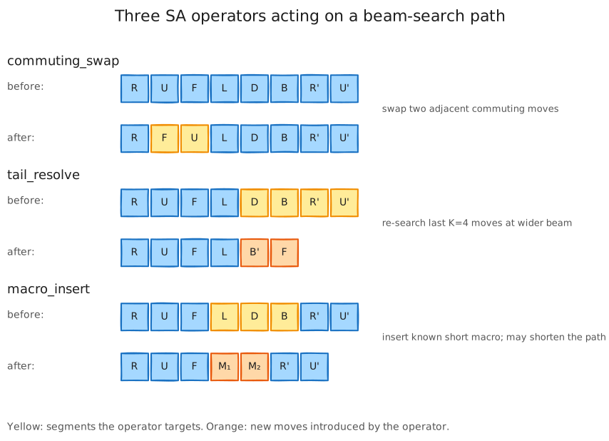
It took ~36 hours on a single L4 to run the SA pass on the top-200 longest paths. 122 of them were improved for 471 moves in total.
The next steps were about pushing post-processing further, adding small tricks and min-merging solutions together with other competition participants.
What working with Claude looks like
As I have mentioned before, I usually set direction and let Claude implement everything.
Where Claude worked well
- Auto-research for model improvement and ablations on possible issues. Claude was able to suggest improvements to the model, run them, and do the next steps. When it implemented multiple changes at once and the results were worse, it ran ablations to isolate the issue.
- Code velocity. Creating working code took much less time than writing it by hand.
- Paper or idea implementation. It was easy to tell Claude to implement a specific paper or idea; it usually did so relatively well.
- Training on different hardware. I trained locally on a 4090, on Kaggle, and on a GCP GPU - Claude easily managed it.
- Documentation. I asked Claude to document every single experiment, decision, and idea. It helped reproduce previous solutions and avoid getting lost in the sheer volume of tried ideas.
Where Claude failed
- Endless iterations without significant improvements. The agent was happy to try dozens of small ideas that didn’t improve the results or to train many models for blending.
- Using non-optimal hardware for wrong reasons. Claude sometimes launched long processes on my local laptop that could take 1-2 days rather than using GCP or Kaggle.
- Being unable to find novel ideas. Most of the significant improvements came from my nudging, not from it itself.
Conclusion
This was my first time using agents for working on a long-term research project. It took me ~4–6 weeks of iteration to implement everything described in this post, and the main time sink was waiting for model training and beam search. Without using Claude, it would have taken me many months to implement everything, and I would have spent a lot of time on debugging and implementation details.
I was surprised how much of the implementation work could be delegated to an agent, and how much time it saved me. I was also surprised how much of the research work still required human intuition and creativity. The agents can’t handle ambiguity well and often prefer to follow safer ideas (despite being asked to be “bold”). But I’m sure the agents will become better in the future. The main benefit for me was that the cost of trying an idea has dropped enough that the bottleneck is now the ideas themselves. But that works only if you keep the agent on a tight leash and don’t let it pursue wrong ideas or avoid implementing complex ideas.
Working with Cayley graphs is a fascinating area of research, and I hope this post inspires others to explore it. If you are interested in this project, you are welcome to participate in the Kaggle competitions IHES Picture Cube and Megaminx. These competitions are useful because they turn abstract group searches into an engineering benchmark. Every improvement shows up as shorter paths and a better leaderboard score.
blogpost datascience kaggle competition ai claude agent