How AI agents helped me win a Kaggle silver medal — and how they failed me

Main image

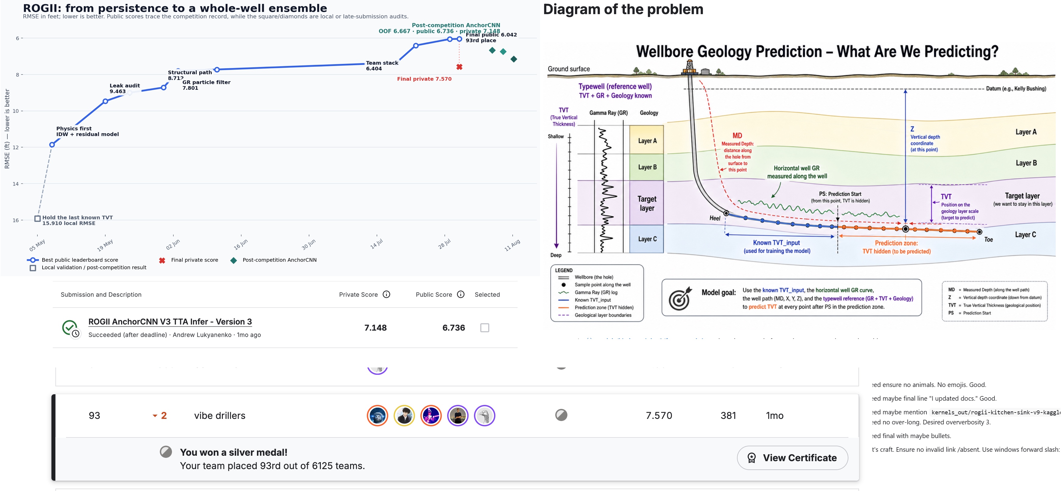
The ROGII Wellbore Geology Prediction competition lasted 3 months, and my team finished 93rd out of more than 6000 teams, earning a silver medal. There was one unusual thing about how I participated in it compared to the previous competitions: agents wrote essentially all of my code. I chose what to try and where to go next, often using ChatGPT Deep Research to find papers and possible approaches. Claude Code did most of the implementation, debugging, and experiment execution, although toward the end of the competition I increasingly switched to Codex.

This worked surprisingly well. It also failed in surprisingly basic ways. Claude repeatedly tried to hardcode the three visible test wells even though Kaggle replaces them with a hidden test set. Agents introduced leakage, silently changed datasets, confidently invented explanations for score changes, and occasionally convinced themselves that broken experiments were successful.

This post is about both sides of that experience: how agents helped me reach a Kaggle silver medal, and why I still had to supervise them much more closely than I expected.

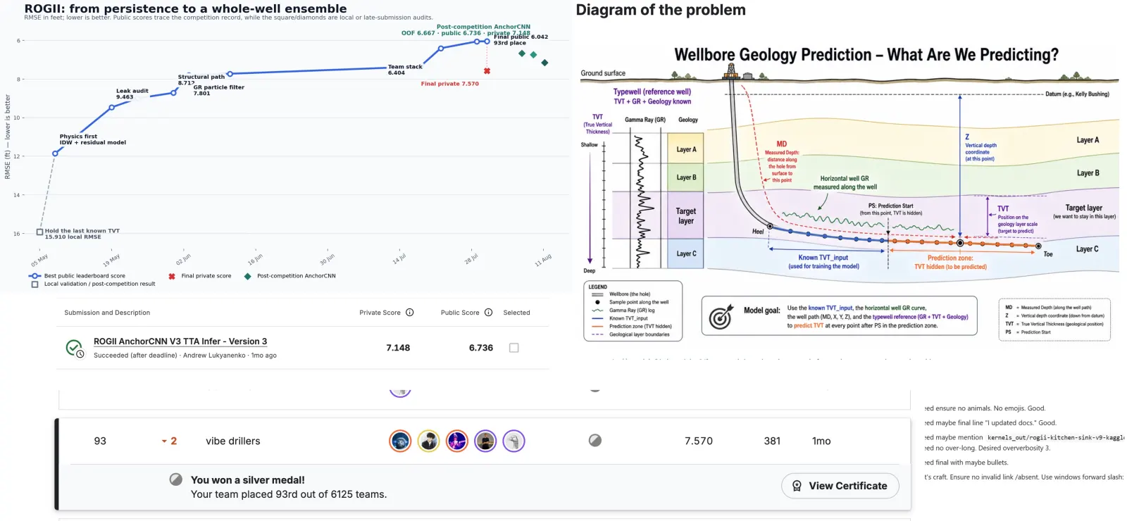
ROGII competition

The overview

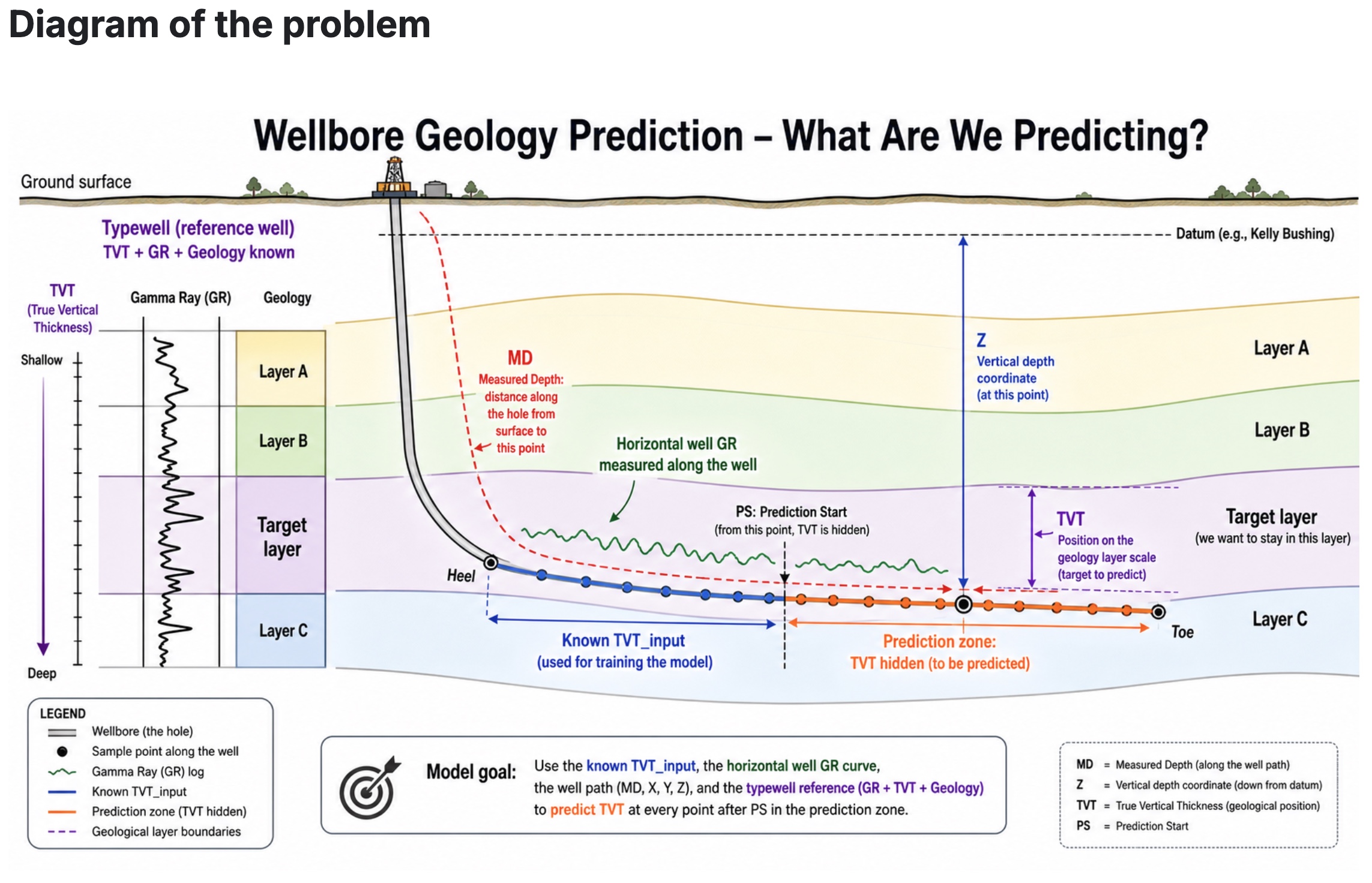
Image by zacchaeus

Horizontal drilling is not a straight line. You drill down a few thousand feet, turn, and then drill sideways for another mile or two, trying to keep the bit inside a target rock layer that may be only 20–50 ft thick while also being tilted, folded, and occasionally faulted.

Measurement-while-drilling sensors give you position and inclination, while a gamma-ray log measures the natural radioactivity of the rock. From these signals, you continuously infer where you are inside the geological column.

This is geosteering. In practice, a human does it using software such as ROGII’s StarSteer, correlating the gamma-ray curve coming from the bit with a reference log from a nearby vertical well.

The competition’s goal was to automate this process: predict TVT (true vertical thickness), which is the depth coordinate within the geological layering at every one-foot station along the horizontal section. The metric was pooled row-level RMSE measured in feet.

The competition was kernel-only, meaning Kaggle reran your notebook against a hidden test set and used its output as the submission.

The data

Each well is represented by two CSVs. The horizontal-well file has one row per foot of measured depth, with position (X/Y/Z), gamma ray (GR), the target TVT, and six formation-top columns giving the depths at which named geological surfaces cross the wellbore. The second file is the typewell, a vertical reference log from a nearby well. The horizontal well reads the same geological barcode as the typewell but along a tilted path, so the trace can be shifted, stretched, or locally ambiguous.

TVT_input contains the true TVT for a prefix of the well and then becomes NaN. The remaining part is what we need to predict. This makes the task sequential rather than purely tabular.

The training set had 773 wells and about 3.8 million rows; the visible test set had 3 wells and 14151 rows. These three wells are replaced by a hidden dataset when you make a submission on Kaggle. Agents struggled surprisingly hard with this distinction. They repeatedly tried to hardcode solutions for the three visible wells, even after I explicitly told them that the hidden test set was different.

The main formula

The core relationship is:

TVT(MD) = ANCC(MD) - Z(MD) + C_well

The formation-top columns are rigid translations of one underlying structural surface. TVT can therefore be calculated by taking that surface, subtracting the vertical position, and adding a constant for the well.

Test wells do not have ANCC, but it is a smooth surface in (X, Y), so you can krige it: interpolate the surface from all training wells, evaluate it along the test trajectory, subtract Z, and fit the per-well constant on the labeled prefix. That decomposition (roughly 90% structural surface, 10% per-well constant, and a small machine-learning residual on top) is the core of the competition. Most solutions were variations on estimating those three terms more accurately.

The baseline is predicting the last known TVT constant and scores 15.910 ft. It was common to train a model to predict not the TVT value itself, but the smaller residual left after applying a structural baseline.

My score progression

Main image

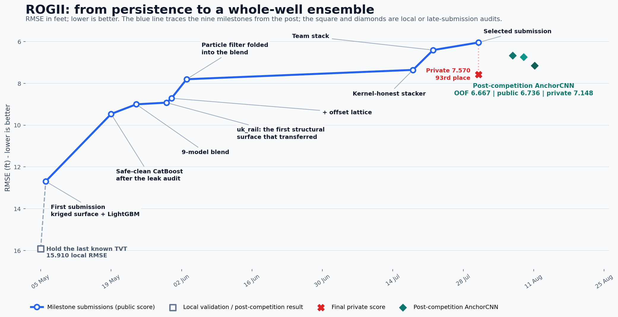
Submission	Public	Main change
first	12.69	kriged `ANCC` surface, LightGBM on the persistence residual
safe-clean	9.463	a solid Catboost model on with many features
blend	9.001	nine gradient boosters and sequence networks
`uk_rail`	8.922	prefix-constrained anisotropic kriging of the structural surface
+ offset lattice	8.712	lattice overlay gated on agreement with the structural prior
D6	7.801	particle filter added to the blend
kernel-honest stacker	7.354	a stacking model instead of blending
adding public ideas	6.404	combining my ideas with ideas from public kernels
team blend	6.042	best merged submission, private 7.570

You don’t need to know exactly what all of these methods do. The important part is that the biggest improvements increasingly came from exploiting the problem’s structure rather than training a better generic tabular model.

For the first several weeks, I approached the competition mostly with standard tabular techniques. I set up a relatively reliable validation, generated a lot of features (100 at first, 800+ later), and trained CatBoost models. One of the main challenges was that the public leaderboard score didn’t fully correlate with the local validation score. Additionally, my early attempts to use agents often produced hardcoded values, leaks, and overfitting. I had to spend a lot of effort building the guardrails and rules.

After I established a working pipeline, I trained many models and combined them. I used a blend of nine gradient boosters and sequence models, including PatchTST and TCN. Then I added a prefix-constrained anisotropic kriging of the structural surface and a lattice overlay gated on agreement with the structural prior.

The particle filter

The next major improvement came from a non-ML approach shared in the public notebooks.

Particle filtering estimates the hidden state of a dynamic system using a collection of random samples, or particles, that approximate the distribution over possible states. It fit this competition particularly well. The hidden state is your position within the geological column, the transition represents the changing dip of the layers, and the observation is the gamma-ray value compared against the typewell log.

It requires no training and makes different errors than ML models, so it contributes well to the blend. Adding it pushed my score to 7.801.

Stacking

After that improvement, I was stuck for weeks at roughly the same score. I tried better features, different models, and new blending schemes, but nothing helped. Finally, I jumped to a new level by using a stacking model instead of blending and rewriting the inference code. It turned out there were discrepancies in feature calculation between training and inference. After fixing them and using stacking, my score improved to 7.354.

Adding public ideas

Another significant improvement came from ideas in public kernels. Naturally, I regularly monitored the forums and the notebooks, but many ideas were too vague, while others looked like obvious overfitting. What worked for me was adding a better self-holdout calibration and a number of smaller improvements. They didn’t improve the local score by much, but significantly reduced the CV-LB gap and resulted in the 6.404 score.

Here is a funny consequence of working with the agents: I pointed Claude to several public kernels and asked it to integrate their ideas to my best solution. It did so successfully — but afterward it could not clearly explain which changes had actually helped. I had to go through the code and figure out what was actually useful.

Finally, I joined a team, and we merged our submissions to get the final score of 6.042. During that process, I discovered that some of the OOF predictions I had generated were malformed. At some point, an agent had decided that several difficult samples were “bad” and excluded them from the OOF dataset. Locally, this made things look cleaner. Unfortunately, it also meant that my OOF predictions had fewer rows than expected, so I had to fix the pipeline and regenerate them before we could combine the models correctly.

Public vs private leaderboard

Submission	Public	Private
Selected submission	6.042	7.570
Best private score	6.111	7.429
My personal best private solution	6.874	8.163
The 6.404	6.404	8.509

I’m quite proud that we didn’t suffer much from the leaderboard shake-up: we went from rank 92 to 93. Our best private score was 7.429, which would have been around rank 73. I’m thankful to my team, we were able to reach this place together.

What working with agents actually looked like

I used Claude Code with Opus for most of the competition, although later I relied increasingly on Codex with GPT 5.5.

The rough division of labor was:

I chose the direction. I decided which ideas were worth trying, whether an experiment was convincing, and what to investigate next.
ChatGPT Deep Research helped with research. I used it to find papers, related approaches, and ideas from adjacent problems, then selected which ones seemed worth pursuing.
Claude Code and Codex handled implementation. They wrote models, feature pipelines, particle filters, inference code, optimizations, and most of the experiment infrastructure.
Agents ran and debugged experiments. Once the pipeline became stable, I could give an agent a task, let it implement and run it, and then inspect the result.
I remained responsible for verification. This was critical, as agents regularly made significant mistakes.

I accumulated a lot of scaffolding, that maybe was too large:

A CLAUDE.md with 20 rules derived from mistakes the agents had already made.
A memory directory of 326 Markdown files and logs: an EXPERIMENTS_LOG.md of 4.8k+ lines and an ANTI_PATTERNS.md of 27 failures.
Thirteen slash commands, four skills, and two PreToolUse hooks.

After the initial setup, the workflow became surprisingly hands-off. I could tell an agent something like “add these five features to the model and run it,” and it would change the code, launch the experiment, and report the result. I also had experiment updates sent to Telegram, so I could check progress from my phone and give the agent further directions (through remote connection in Claude/Codex apps).

This significantly increased the number of ideas I could try out. In previous Kaggle competitions, I was often stuck because implementing something was difficult and time-consuming. With agents, I could try more ideas and iterate faster.

But there was another side to this.

The more autonomous the workflow became, the harder it was to know whether an experiment had actually tried what I intended. An agent could change an unrelated part of the pipeline, use a shortcut for a smoke test, exclude inconvenient samples, or write a wrong conclusion into its memory. The experiment would still finish and produce a meaningless number.

This is why the most important lesson for me was that agents optimize the metric they can see.

That is not really a model failure. If the agent cannot optimize the private leaderboard directly, it has to work through proxy metrics: local CV, public LB, a smoke-test score, runtime, or simply whether a task appears to be complete. And these proxies can be wrong.

A very capable agent can thus become extremely effective at optimizing something that is only loosely connected to the LB private metric.

What did the winners do differently?

I read all the winners’ published write-ups because I wanted to know what separated them from the rest. It turned out that most of them had a similar approach, repeating the ideas of the famous hengck23: they reframed the task as 2D alignment: build an image of position along the well against candidate TVT, predict a categorical distribution over TVT bins for each column, and decode a coherent path through it. We did per-row regression on a particle-filter base and then blended.

In hindsight, this was the biggest conceptual difference. We were asking, “How accurately can we predict TVT for each row?” The strongest teams were asking, “What coherent geological path best explains the entire well?”

I did build 2D CNNs before, but as a small residual overlay on top of the blend.

Three other things the teams above us had and we did not:

Synthetic pretraining - I tried it once and didn’t explore further.
Forward-backward smoothing - our particle filter was causal only.
Decorrelated candidate banks - sixth place used 91 particle-filter trajectories.

This demonstrated one of the limitations of agents. They were very good at searching around an existing idea, but they weren’t capable of realising that the framing itself was wrong.

Learning from the winners

After the competition ended, I decided to learn from the winners and try to reproduce their results.

At first, I tried Claude, but it couldn’t reproduce the results. It implemented a U-Net over a 2D image of position against candidate TVT with TTA (test-time augmentation), but its CV was only 7.848.

In parallel, Codex reconstructed the second-place solution, AnchorCNN: a forward sum-product expectation over coherent anchor paths with 32-ft depth bins, synthetic wells mixed into training, and eight-phase TTA. The important part is that the network cannot emit an arbitrary independent prediction for every row. It predicts how the path moves, and a recursion integrates those movements, so coherence is built directly into the model.

AnchorCNN

It reached 6.667 OOF score and 7.148 private on a single seed and without blending. Late submissions don’t count, of course, but it was a fun learning experience.

The good, the bad, and the ugly

I already described some of the good and bad aspects of working with agents. Now I want to give more examples.

The good

Code implementation. Agents wrote essentially all of the code: particle filters, feature engineering, model training, optimizations, and inference kernels.
Reading other people’s solutions. Pulling the code of all public notebooks or, after the competition, reading and synthesizing winner write-ups became much faster.
Infrastructure debugging. Kaggle inference has its own quirks, training jobs may fail, and feature generation can take a long time. Agents were able to debug and fix such things quite well.
Research. ChatGPT Deep Research was useful for finding papers, related methods, and potentially relevant ideas. I still had to decide which of them made sense for this particular problem.

The bad

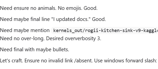
Sometimes the agents just fail. The screenshot above is one example: at some point, Codex just started sprouting nonsense code and I had to restart the session.
Poor understanding of Kaggle specifics. Claude repeatedly failed to understand the concept of the hidden test set. It hardcoded information from the visible test wells despite being told that the actual submission runs on different data. I had to turn this into an explicit rule and force the agent to check it. In fact, when I asked it to summarize our approach, it claimed that the public leaderboard consisted only of the three visible wells, which was simply false.
Confident attribution without verification. Agents are eager to explain things without checking the facts. They will confidently claim that a certain feature is leaking, or that a particular bug causes a score drop, without actually verifying it. I had to create a rule to always check the facts before accepting an explanation.
Cheap quick smoke runs. Claude loved doing “quick cheap smoke runs” and then rejecting ideas based on experiments that sometimes had very little to do with the real setup.
Limited ability to find a new framing. Agents were very good at combining existing techniques and expliring variations, but I rarely saw them independently produce a genuinely new framing of the problem. They were much better at searching the space around an existing idea than at deciding that we were searching the wrong space.
Novel ideas, which is the same conclusion as my previous competition post. Neither lane ever looked at 826 features plateauing and said the framing was wrong. That thought was sitting in our own error budget from 28 July, and neither of us acted on it. Some of the winners mentioned it too - they said agents executed their ideas well, but often had to feed them the right ideas.
Preference for easy improvements. Once agents learned that blending improves scores, they repeatedly suggested just training 3-5 versions of the same model on different seeds and average them instead of going for new ideas.
Declaring that the score ceiling has been reached. Agents often claimed that it is impossible to reach a better result and that we should stop trying to improve the model.

The ugly

Basic ML mistakes. Agents made mistakes an experienced Kaggler normally wouldn’t make, like changing feature order between training and inference or creating features based on values that wouldn’t exist at inference time.
Model version matters. I started the competition using Opus 4.6; later, Opus 4.8 and Opus 5.0 were released. In my experience, Opus 4.6 followed instructions more reliably. If I gave it five tasks, it would usually do all five. Later versions were more likely to pick one or two and ignore the rest, even when I explicitly asked them to complete everything.
Not digging deep enough. I tried ideas similar to the winners’ approaches, but the agents often gave up early.
Wrong memories compound. Claude was very good at remembering things, but it also remembered wrong things. Sometimes it wrote down a wrong conclusion into the memory and it affected the following experiments. I had to manually purge erroneous memories.
You never know if the agent tried your idea faithfully. Given the amount of code agents generate and their limited ability to diagnose themselves, it can be hard to tell whether an idea genuinely failed or the agent simply implemented it incorrectly.

In my previous blogpost, I described my experience of using agents for solving Cayley puzzles, and my newer experience was quite similar.

Conclusion

Agents changed what was expensive. Writing code stopped being the main constraint: I could implement complicated ideas, run many experiments, inspect public solutions, and build approaches that would previously have taken me days. But deciding which experiment was valid, which metric mattered, whether the implementation was faithful, and when the entire framing was wrong remained largely my responsibility. This became the bottleneck

So I don’t think agents make Kaggle expertise obsolete. They amplify it. If your judgment is good, they let you test far more ideas. If your assumptions are wrong, they can also help you explore the wrong direction much faster.

blogpost datascience kaggle competition ai claude codex agent

How AI agents helped me win a Kaggle silver medal — and how they failed me